Simulation

In this section we will discuss the topic of simulating feedback control systems and provide a simulation framework that was built during this study. We will later use this framework in a couple of case studies.

There are a number of reasons why we need the ability to simulate the behavior of a control system.

• First of all, the behavior of a control system might be unintuitive or unfamiliar. To develop intuition for the abstract problem we can use simulations and thus get a better understanding of control problems that arise in the real world.
• In most cases it is not possible to do extensive testing and experimenting on real-world machines. Often they are too big, too expensive, too dangerous or simply not available. And if they are available, tests will mostly be too time consuming to conduct serious experiments. Therefore simulations will suit better.
• The most difficult part is to implement controllers, filters, etc. according to abstract concepts like transfer functions. Simulations can help with a better understanding and make these concepts more concrete.
• Finally, no control system will ever be put into production unless it has proven itself to function correctly. Therefore, simulations are not just for fun, but form a crucial step in the design of a feedback control system.

In this section of the blog we will discuss a simulation framework that was built for this study. Also we will go over a number of case studies by using this framework.

Time

One of the most important parts of the simulation framework is the simulation of time. For computer systems we are given with a choice between two possible representations. We can use real time (also known as 'wall-clock' time) where the controlled system evolves according to its own rules and dynamics, independent from control actions. In this case, control actions will usually occur periodically with a fixed time interval between two actions. Another choice is to use control time (also known as 'event time'). Here the system does not evolve between two control actions, hence the time is synchronous with the control actions. Notice that this is the type of time that was used in the earlier examples.

In a simulation, the time is determined by the number of simulation steps. To convert this to a simulation of real time, we must assume that each simulation step has exactly the same duration (measured in real time). Therefore the steps in the simulation correspond to a certain duration in real time. Hence we need a conversion factor DT that translates simulation steps into real time durations.

Simulation framework

In order to model every component in the simulation framework, we use a Component trait (or interface) containing two abstract functions: update and action. The former is used to iterate to the component's state in the next simulation step, based on its current state and an update parameter u. The latter is used to calculate the action that needs to be taken at the current simulation step. To see what is going on inside a component, another abstract function monitor is provided that returns a Map[String, AnyVal]. This needs to be implemented on each component.

Furthermore it should be noticed that components can be concatenated in order to compose more complex components. In other words, Component can be viewed as a monoid, hence the ++ operator. Also, we can implement map on a Component in order to apply functions to the output signal of a component (Component is a functor).

trait Component[I, O] {
    def update(u: I): Component[I, O]
    def action: O
    def monitor: Map[String, AnyVal]

    def ++[Y](other: Component[O, Y]): Component[I, Y] = {
        val self = this
        new Component[I, Y] {
            def update(u: I): Component[I, Y] = {
                val thisComp = self update u
                val otherComp = other update thisComp.action
                thisComp ++ otherComp
            }

            def action: Y = other.action
        }
    }

    def map[Y](f: O => Y): Component[I, Y] = {
        val self = this
        new Component[I, Y] {
            def update(u: I): Component[I, Y] = self update u map f

            def action: Y = f(self action)

            def monitor = self.monitor
        }
    }
}

Controller

Controllers convert the tracking error in a system input. As discussed before, the most common controller is the PIDController. Here update calculates the new integral and derivative components of this controller and returns a new instance with these new values, whereas action calculates the value of the control action, which serves as an input for the controlled system. Notice that here the earlier discussed DT factor enters the calculations twice.

class PIDController(kp: Double, ki: Double, kd: Double = 0.0, integral: Double = 0, deriv: Double = 0, prev: Double = 0)(implicit DT: Double) extends Component[Double, Double] {
    def update(error: Double): PIDController = {
        val i = integral + DT * error
        val d = (error - prev) / DT

        new PIDController(kp, ki, kd, i, d, error)
    }

    def action = prev * kp + integral * ki + deriv * kd

    def monitor = Map("PID controller" -> action)
}

A more advanced implementation can be found in AdvController, which adds two features to PIDController. First it has a filter for smoothing the derivative term. Supplying a positive value 0 < s < 1 will result in applying a recursive filter on the derivative term. Furthermore a parameter clamp is added, which prevents integrator windups. This means that when the controller's output exceeds a certain limit (defined by clamp), the controller will not update its value during the next round.

Regarding the latter feature, this controller can be used to control a heating element. Here a lower bound can be set on 0° Celsius, since it is usually impossible for a heating element to produce negative heat flow.

class AdvController(kp: Double, ki: Double, kd: Double = 0, clamp: (Double, Double) = (-1e10, 1e10), smooth: Double = 1, integral: Double = 0, deriv: Double = 0, prev: Double = 0, unclamped: Boolean = true)(implicit DT: Double) extends Component[Double, Double] {
    def update(error: Double): AdvController = {
        val i = if (unclamped) integral + DT * error else integral
        val d = smooth * (error - prev) / DT + (1 - smooth) * deriv

        val u = kp * error + ki * integral + kd * deriv
        val un = clamp._1 < u && u < clamp._2

        new AdvController(kp, ki, kd, clamp, smooth, i, d, error, un)
    }

    def action = prev * kp + integral * ki + deriv * kd

    def monitor = Map("Advanced controller" -> action)
}

Filters and actuators

Besides controllers, we also might want to make use of other components. These are the actuators and filters. The most obvious one (Identity) just reproduces its input value and emits that as its output.

class Identity[A](value: A = 0) extends Component[A, A] {
    def update(u: A): Identity[A] = new Identity(u)

    def action = value

    def monitor = Map("Identity" -> action)
}

Another actuator is the Integrator, which takes the sum of its inputs and returns its current value. Notice that since we are calculating an integral here and that therefore we need to multiply the sum by factor DT to convert from simulated steps to real time.

class Integrator(data: Double = 0)(implicit DT: Double) extends Component[Double, Double] {
    def update(u: Double): Integrator = new Integrator(data + u)

    def action = DT * data

    def monitor = Map("Integrator" -> action)
}

Finally we present two smoothing filters. The first, FixedFilter, calculates the unweighted average of the last n elements.

class FixedFilter(n: Int, data: List[Double] = List()) extends Component[Double, Double] {
    def update(u: Double): FixedFilter = {
        val list = (if (data.length >= n) data drop 1 else data) :+ u
        new FixedFilter(n, list)
    }

    def action = data.sum / data.length

    def monitor = Map("Fixed filter" -> action)
}

The second filter, RecursiveFilter is an implementation of the exponential smoothing algorithm. This adds the current value u to the previous filter output in order to return the current step's output.

class RecursiveFilter(alpha: Double, y: Double = 0) extends Component[Double, Double] {
    def update(u: Double): RecursiveFilter = {
        val res = alpha * u + (1 - alpha) * y
        new RecursiveFilter(alpha, res)
    }

    def action = y

    def monitor = Map("Recursive filter" -> action)
}

Convenience functions

Finally we introduce a number of convenience functions with the intention of hiding most of the boilerplate code. First we have a number of basic setpoint functions. These can be used as input for a feedback loop, but can also be composed to get a more complex setpoint function by multiplying the result of such a function with a scalar and/or adding with other functions.

object Setpoint {
    def impulse(t: Long, t0: Long)(implicit DT: Double) = {
        if (math.abs(t - t0) < DT) 1
        else 0
    }

    def step(t: Long, t0: Long) = {
        if (t >= t0) 1
        else 0
    }

    def doubleStep(t: Long, t0: Long, t1: Long) = {
        if (t >= t0 && t < t1) 1
        else 0
    }

    def harmonic(t: Long, t0: Long, tp: Long) = {
        if (t >= t0) math.sin(2 * math.Pi * (t - t0) / tp)
        else 0
    }

    def relay(t: Long, t0: Long, tp: Long) = {
        if (t >= t0 && math.ceil(math.sin(2 * math.Pi * (t - t0) / tp)) > 0) 1
        else 0
    }
}

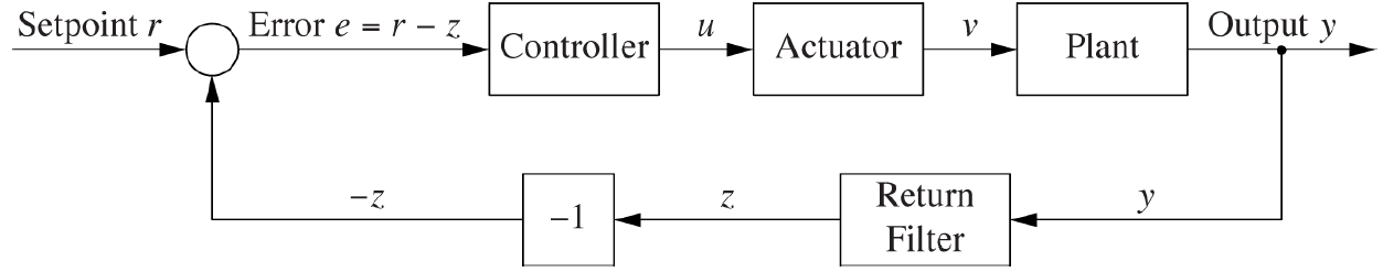
Also we provide the boilerplate code for multiple types of loops. For now we discuss the closedLoop and come back later to other types of loops. This function is modeled after the extended version of a feedback control system, including the actuator and filter.

object Loops {
    def closedLoop[A](setPoint: Observable[A], seed: A, components: Component[A, A], inverted: Boolean = false)(implicit n: Numeric[A]) = {
        import n._
        Observable[A](subscriber => {
            val y = BehaviorSubject(seed)
            y drop 1 subscribe subscriber

            setPoint.zipWith(y)(_ - _)
                .map { error => if (inverted) -error else error }
                .scan(components)(_ update _)
                .drop(1)
                .map(_ action)
                .subscribe(y)
        })
    }
}

Notice that using the closedLoop function on a control system with controller, actuator, plant (the controlled system) and filter will require using the ++ operator in order to concatenate these components.

Running example

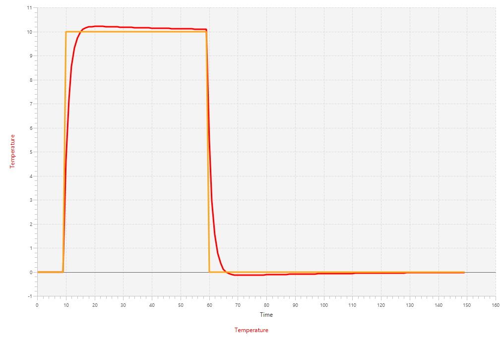
To demonstrate the workings of these basics, let's implement a simple plant Boiler and see how this framework performs:

class Boiler(g: Double = 0.01, y: Double = 0)(implicit DT: Double) extends Component[Double, Double] {
    def update(u: Double) = new Boiler(g, y + DT * (u - g * y))

    def action = y

    def monitor = Map("Boiler" -> action)
}

Then we can use this plant to create a small example program. We first initialize the DT variable (default to 1.0) and construct a setpoint function from one of the convenience functions as well as the time, plant and controller. Finally we put these all in the closedLoop function and print the result.

def simulation(): Observable[Double] = {
    implicit val DT = 1.0
    def setpoint(t: Long): Double = 10 * Setpoint.doubleStep(t, 10, 60)

    val time = (0L until 150L) toObservable
    val p = new Boiler
    val c = new PIDController(0.45, 0.01)

    Loops.closedLoop(time map setpoint, 0.0, c ++ p)
}

The results of running this example program will yield the following plot: